George Mason University
OR 538
R/SYST-538 HOMEWORK-4
Chapter-7
Problem-1
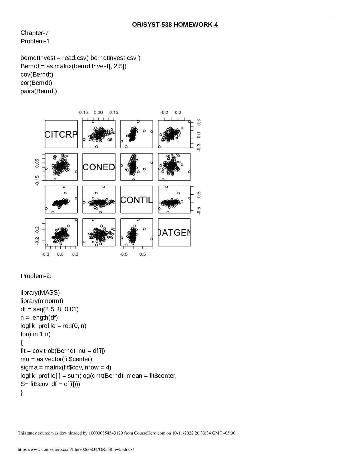
berndtInvest = read.csv("berndtInvest.csv")
Berndt = as.matrix(berndtInvest[, 2:5])
cov(Berndt)
cor(Berndt)
pairs(Berndt)
Problem-2:
library(MASS)
library(mnormt)
df = seq(2.5, 8, 0.01)
n = length(df)
loglik_profile = rep(0, n)
for(i in 1:n)
{
fit = cov.trob(Berndt, nu = df[i])
mu = as.v
...[Show More]
R/SYST-538 HOMEWORK-4
Chapter-7
Problem-1
berndtInvest = read.csv("berndtInvest.csv")
Berndt = as.matrix(berndtInvest[, 2:5])
cov(Berndt)
cor(Berndt)
pairs(Berndt)
Problem-2:
library(MASS)
library(mnormt)
df = seq(2.5, 8, 0.01)
n = length(df)
loglik_profile = rep(0, n)
for(i in 1:n)
{
fit = cov.trob(Berndt, nu = df[i])
mu = as.vector(fit$center)
sigma = matrix(fit$cov, nrow = 4)
loglik_profile[i] = sum(log(dmt(Berndt, mean = fit$center,
S= fit$cov, df = df[i])))
}
Exercise-1
a) E(0.2X + 0.8Y ) = (0.2)(1) + (.8)(1.5) = 1.4
Var(0.2X + 0.8Y ) = (0.2^2)(2) + 2(0.2)(0.8)(0.8) + (0.8^2)(2.7) = 2.064
b) Var{wX + (1 - w)Y }
= 2w^2 + 2w(1 - w)(.8) + (2.7)(1 - w)^2
= 4w + 2(1 - w)(.8) - 2w(.8) - 2(1- w)(2.7)
= (4 - (1.6)(2) + (2)(2.7))w + 1.6 - (2)(2.7)
= 6.2w - 3.8
= 0
w= 0.613
Yes it is useful to minimize the variance since it minimizes the risk.
Chapter-9
Problem-1:
install.packages("AER")
library(AER)
data("USMacroG")
MacroDiff = apply(USMacroG,2,diff)
pairs(cbind(MacroDiff[,c("consumption","dpi","cpi","government","unemp")]))
There are no outliers in the plot. For predicting changes in consumption we have to use predictors
that have least correlation. Among the all unemp and dpi seem to have very less correlation henc
[Show Less]