University of British Columbia STAT 443 stat443-final2018
1. From the R data set Seatbelts, we have the monthly number of rear passengers killed in automobile
accidents from January 1969 to December 1984. Below is the plot of the decomposition function,
decompose() in R, assuming an additive model, which shows the observed time series, the trend
component (mb t), the seasonal component (¯
...[Show More]
University of British Columbia STAT 443 stat443-final2018
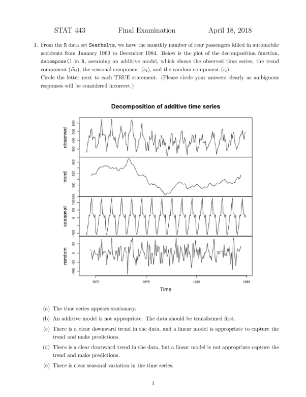
1. From the R data set Seatbelts, we have the monthly number of rear passengers killed in automobile
accidents from January 1969 to December 1984. Below is the plot of the decomposition function,
decompose() in R, assuming an additive model, which shows the observed time series, the trend
component (mb t), the seasonal component (¯ st), and the random component (�t).
Circle the letter next to each TRUE statement. (Please circle your answers clearly as ambiguous
responses will be considered incorrect.)
(a) The time series appears stationary.
(b) An additive model is not appropriate. The data should be transformed first.
(c) There is a clear downward trend in the data, and a linear model is appropriate to capture the
trend and make predictions.
(d) There is a clear downward trend in the data, but a linear model is not appropriate capture the
trend and make predictions.
(e) There is clear seasonal variation in the time series.
[Show Less]


-preview.png)