Toronto Metropolitan University

GMS 804

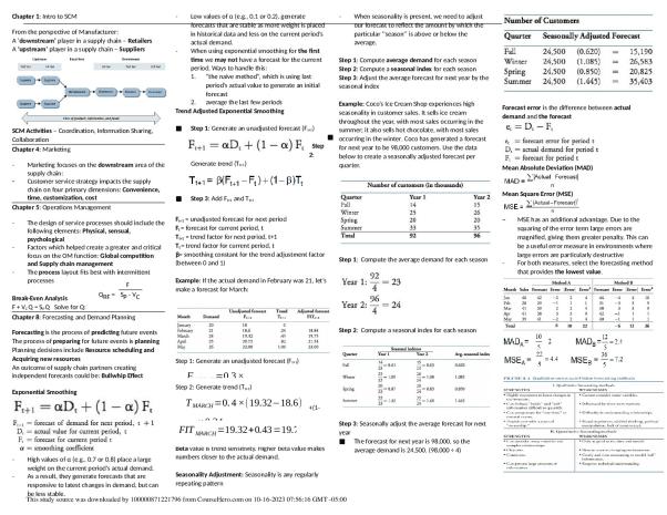
Chapter 1: Intro to SCM
From the perspective of Manufacturer:
A ‘downstream’ player in a supply chain – Retailers
A ‘upstream’ player in a supply chain – Suppliers
SCM Activities – Coordination, Information Sharing,
Collaboration
Chapter 4: Marketing
- Marketing focuses on the downstream area of the
supply chain:
- Customer service strategy impacts the supply
chain on four primary dimensions: Convenience,
time, customization, cost
Chapter 5: Operations Management
- The design of service processes should include the
following elements: Physical, sensual,
psychological
- Factors which helped create a greater and critical
focus on the OM function: Global competition
and Supply chain management
- The process layout fits best with intermittent
processes
Break-Even Analysis
F + VC Q = SP Q Solve for Q:
Chapter 8: Forecasting and Demand Planning
Forecasting is the process of predicting future events
The process of preparing for future events is planning
Planning decisions include Resource scheduling and
Acquiring new resources
An outcome of supply chain partners creating
independent forecasts could be: Bullwhip Effect
Exponential Smoothing
- High values of α (e.g., 0.7 or 0.8) place a large
weight on the current period’s actual demand.
- As a result, they generate forecasts that are
responsive to latest changes in demand, but can
be less stable.
- Low values of α (e.g., 0.1 or 0.2), generate
forecasts that are stable as more weight is placed
in historical data and less on the current period’s
actual demand.
- When using exponential smoothing for the first
time we may not have a forecast for the current
period. Ways to handle this:
1. “the naive method”, which is using last
period’s actual value to generate an initial
forecast
2. average the last few periods
Trend Adjusted Exponential Smoothing
■ Step 1: Generate an unadjusted forecast (Ft+1)
■
Step
2:
Generate trend (Tt+1)
■ Step 3: Add Ft+1 and Tt+1
Ft+1 = unadjusted forecast for next period
Ft = forecast for current period, t
Tt+1 = trend factor for next period, t+1
Tt = trend factor for current period, t
β= smoothing constant for the trend adjustment factor
(between 0 and 1)
Example: If the actual demand in February was 21, let’s
make a forecast for March:
Step 1: Generate an unadjusted forecast (Ft+1)
Step 2: Generate trend (Tt+1)
Step 3: Add Ft+1 and Tt+1
Beta value is trend sensitivity. Higher beta value makes
numbers closer to the actual demand.
Seasonality Adjustment: Seasonality is any regularly
repeating pattern
- When seasonality is present, we need to adjust
our forecast to reflect the amount by which the
particular ‘‘season’’ is above or below the
average.
Step 1: Compute average demand for each season
Step 2: Compute a seasonal index for each season
Step 3: Adjust the average forecast for next year by the
seasonal index
Example: Coco’s Ice Cream Shop experiences high
seasonality in customer sales. It sells ice cream
throughout the year, with most sales occurring in the
summer; it also sells hot chocolate, with most sales
occurring in the winter. Coco has generated a forecast
for next year to be 98,000 customers. Use the data
below to create a seasonally adjusted forecast per
quarter.
Step 1: Compute the average demand for each season
Step 2: Compute a seasonal index for each season
Step 3: Seasonally adjust the average forecast for next
year
■ The forecast for next year is 98,000, so the
average demand is 24,500. (98,000 ÷ 4)
Forecast error is the difference between actual
demand and the forecast
Mean Absolute Deviation (MAD)
Mean Square Error (MSE)
– MSE has an additional advantage. Due to the
squaring of the error term large errors are
magnified, giving them greater penalty. This can
be a useful error measure in environments where
large errors are particularly destructive
- For both measures, select the forecasting method
that provides the lowest value