University of Michigan
NAVARCH 565
ROB 535 HW 1 Solution
Prof. Johnson-Roberson and Prof. Vasudevan
9 Oct, 2019
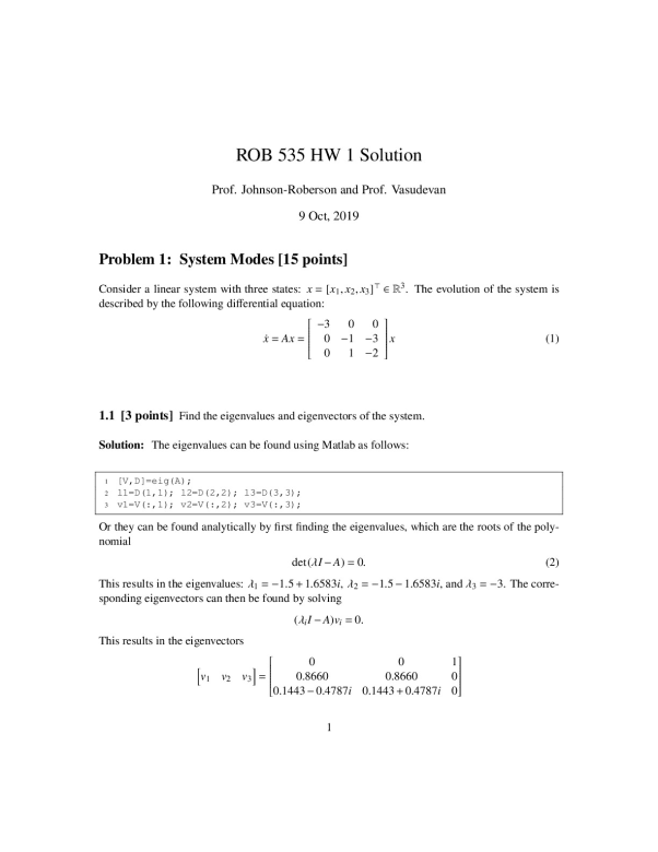
Problem 1: System Modes [15 points]
Consider a linear system with three states: x = [x1; x2; x3]> 2 R3. The evolution of the system is described by the following differential equation:
x˙ = Ax =
0 -1 -3
...[Show More]
ROB 535 HW 1 Solution
Prof. Johnson-Roberson and Prof. Vasudevan
9 Oct, 2019
Problem 1: System Modes [15 points]
Consider a linear system with three states: x = [x1; x2; x3]> 2 R3. The evolution of the system is described by the following differential equation:
| x˙ = Ax = |
0 -1 -3x |
(1) |
| -3 |
0 |
0 |
| 0 |
1 -2 |
2666666664
3777777775
1.1 [3 points] Find the eigenvalues and eigenvectors of the system.
Solution: The eigenvalues can be found using Matlab as follows:
1 [V,D]=eig(A);
2 l1=D(1,1); l2=D(2,2); l3=D(3,3);
3 v1=V(:,1); v2=V(:,2); v3=V(:,3);
Or they can be found analytically by first finding the eigenvalues, which are the roots of the polynomial
det(λI - A) = 0: (2)
This results in the eigenvalues: λ1 = -1:5+1:6583i; λ2 = -1:5 - 1:6583i; and λ3 = -3. The corresponding eigenvectors can then be found by solving
(λiI - A)vi = 0:
This results in the eigenvectors
hv1 v2 v3i =
2666666664
0:1443-0:4787i 0:1443+0:4787i 0
3777777775
1
(Note: while the autograder doesn’t care what order the eigenvalues are in, it does matter that vi is the corresponding eigenvector to λi.)
1.2 [3 points] Notice that there is one real eigenvector. With symbolic MATLAB, write an expression for the solution x(t) to (1) when
x(0) =
2666666664
500
3777777775
Solution: The solution to the differential equation is
x(t) =
2666666664
500
3777777775
e-3t:
This can be written symbolically in matlab as
1 syms t
2 x=[5;0;0]*exp(-3*t)
1.3 [4 points] Numerically solve (using ode45) for the trajectory x(t) when the system starts from x(0). Let the time span be t 2 [0;10] [s] with ∆t = 0:1 [s].
x(0) =
2666666664
012
3777777775
It may be useful to plot your results as a sanity check.
Solution:
1 f=@(t,x) A*x;
2 tspan=[0:0.1:10];
3 x0=[0;1;2];
4 [T,Y]=ode45(f,tspan,x0);
5 plot(T,Y)
[Show Less]


-by-Gary-Donell-SOLUTIONS-MANUAL-preview.jpeg)
-by-Gary-Donell-INSTRUCTOR’S-SOLUTIONS-MANUAL-preview.jpeg)