CHAPTER 11 EXERCISES 1. Consider the following study: Researchers recorded the temperatures at The Fashion Mall at Keystone in Indianapolis during 40 random days in November and December 2013, then again in June and July 2014. For these same days, they recorded the mall sales. The correlation coefficient between these variables was -0.884 and it was significant a
...[Show More]
CHAPTER 11 EXERCISES
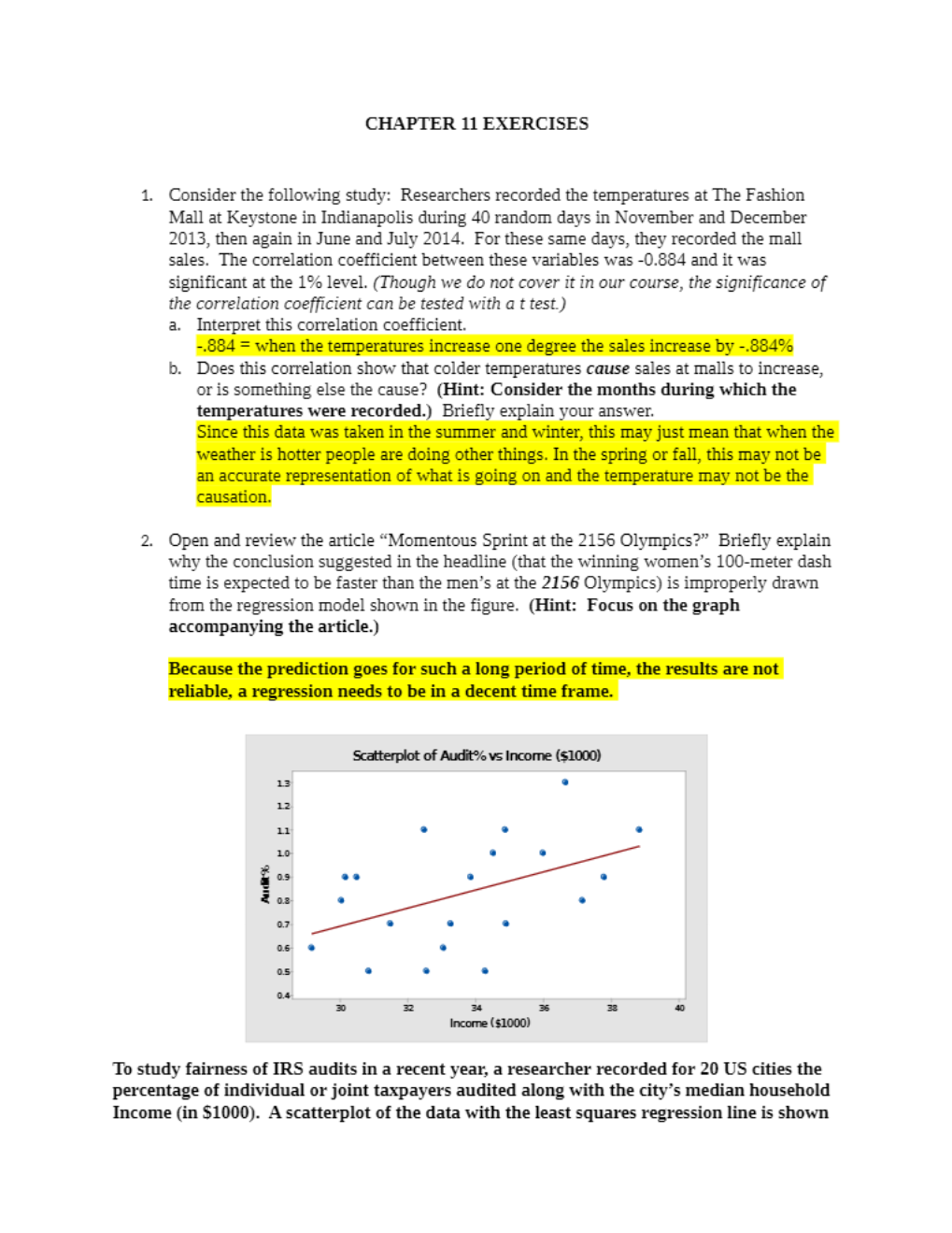
1. Consider the following study: Researchers recorded the temperatures at The Fashion Mall at Keystone in Indianapolis during 40 random days in November and December 2013, then again in June and July 2014. For these same days, they recorded the mall sales. The correlation coefficient between these variables was -0.884 and it was significant at the 1% level. (Though we do not cover it in our course, the significance of the correlation coefficient can be tested with a t test.)
a. Interpret this correlation coefficient.
b. Does this correlation show that colder temperatures cause sales at malls to increase, or is something else the cause? (Hint: Consider the months during which the temperatures were recorded.) Briefly explain your answer.
1. Open and review the article “Momentous Sprint at the 2156 Olympics?” Briefly explain why the conclusion suggested in the headline (that the winning women’s 100-meter dash time is expected to be faster than the men’s at the 2156 Olympics) is improperly drawn from the regression model shown in the figure. (Hint: Focus on the graph accompanying the article.)
To study fairness of IRS audits in a recent year, a researcher recorded for 20 US cities the percentage of individual or joint taxpayers audited along with the city’s median household Income (in $1000). A scatterplot of the data with the least squares regression line is shown above. Below are some basic descriptive statistics for the variables. Questions 3 - 6 concern this data and this regression. Along with noting the correct answer choice, briefly explain all answers.
2. The equation of the least squares regression line to predict Audit% from Income ($1000) is:
A. 0.481 + 0.039(Income)
B. -0.481 + 0.039(Income)
C. 1.477 + 5.614(Income)
D. -1.477 + 5.614(Income)
1. The percentage of variance in the Audit% variable explained by this regression with Income is approximately:
A. 0.466
B. 46.6
C. 21.7
D. 53.4
E. 78.3
1. If Income is recorded in dollars ($) instead of ($1000), the correlation between Audit% and Income ($) will be:
A. 0.000466
B. 0.0466
C. 0.466
D. 0.534
E.
Slide the decimal place over three places.
1. The city with the highest median household income in this dataset is Milwaukee, WI. Its residual in this model is approximately:
A. 0.10
B. -0.10
C. 0.40
D. -0.40
[Show Less]