• George Mason University

• SYST 538  Analytics for Financial Engineering and Econometrics OR/SYST 438/538.  

OR/SYST 438/538: Fall 2016 
I. Chapter 7, Problems #2 (p.178); Exercise #1 (p. 181)
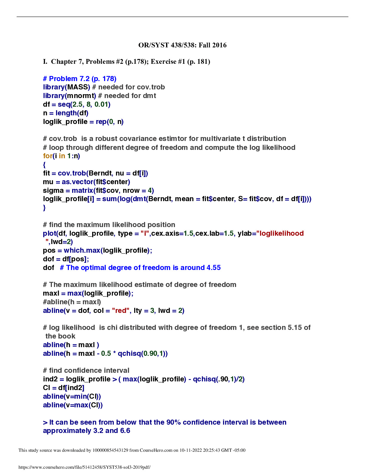
# Problem 7.2 (p. 178)
library(MASS) # needed for cov.trob
library(mnormt) # needed for dmt
df = seq(2.5, 8, 0.01)
n = length(df)
loglik_profile = rep(0, n)
# cov.trob is a robust covariance estimtor for multivariate t distribution
# loop through different degree of freedom and compute the log likelihood
for(i in 1:n)
{
fit = cov.trob(Berndt, nu = df[i])
mu = as.vector(fit$center)
sigma = matrix(fit$cov, nrow = 4)
loglik_profile[i] = sum(log(dmt(Berndt, mean = fit$center, S= fit$cov, df = df[i])))
}
# find the maximum likelihood position
plot(df, loglik_profile, type = "l",cex.axis=1.5,cex.lab=1.5, ylab="loglikelihood
",lwd=2)
pos = which.max(loglik_profile);
dof = df[pos];
dof # The optimal degree of freedom is around 4.55
# The maximum likelihood estimate of degree of freedom
maxl = max(loglik_profile);
#abline(h = maxl)
abline(v = dof, col = "red", lty = 3, lwd = 2)
# log likelihood is chi distributed with degree of freedom 1, see section 5.15 of
the book
abline(h = maxl )
abline(h = maxl - 0.5 * qchisq(0.90,1))
# find confidence interval
ind2 = loglik_profile > ( max(loglik_profile) - qchisq(.90,1)/2)
CI = df[ind2]
abline(v=min(CI))
abline(v=max(CI))
> It can be seen from below that the 90% confidence interval is between
approximately 3.2 and 6.6
 
I. Chapter 7, Exercise #1 (p. 181)
# (a) Given E(x) = 1, E(Y) = 1.5, Var(X) = 2, Var(Y) = 2.7, Cov(X,Y) = 0.8; what are
E(0.2X + 0.8Y ) and Var(0.2X + 0.8Y )?
# E(0.2X + 0.8Y ) = (.2)(1) + (.8)(1.5) = 1.4.
# Var(0.2X + 0.8Y ) = (0.22)(2) + 2(0.2)(0.8)(0.8) + (0.82)(2.7) = 2.064
# (b) For what value of w is Var{wX + (1 - w)Y } minimized? Suppose that X is the
return on one asset and Y is the return on a second asset. Why would it be useful to
minimize Var{wX + (1 - w)Y }?
# Var{wX + (1 - w)Y } = 2w^2 + 2w(1 - w)(.8) + (2.7)(1 - w)^2.
# The derivative of this expression with respect to w is: 4w + 2(1 - w)(.8) - 2w(.8) - 2(1
- w)(2.7) = (4 - (1.6)(2) + (2)(2.7))w + 1.6 - (2)(2.7) = 6.2w - 3.8 = 0 à w= 0.613
# Setting this derivative equal to 0 gives us w = 0.613. The second derivative is positive
so the solution must be a minimum. This means that regardless of the choice of w, that
is, the asset allocation, the risk is minimized at w=0.613. Thus the ratio w = 3.8/6.2
corresponds to the “minimum variance portfolio” (MVP). The corresponding expected
return and variance are: E(wX + (1-w)Y ) = 1.193 with Var(wX + (1-w)Y ) = 1.535
II. Chapter 9, Problems #1,2,3 (p. 244); Exercise #1, #5 (p. 245-246)
# Problem 9.1
# This section uses the data set USMacroG in R’s AER package. This data set contains
quarterly times series on 12 U.S. macroeconomic variables for the period 1950–2000.
We will use the variables consumption = real consumption expenditures, dpi = real
disposable personal income, government = real government expenditures, and unemp
= unemployment rate. Our goal is to predict changes in consumption from changes in
 
the other variables. Run the following R code to load the data, difference the data
(since we wish to work with changes in these variables), and create a scatterplot
matrix.
install.packages("AER")
library(AER)
data("USMacroG")
MacroDiff = apply(USMacroG,2,diff) # apply the diff function on each column
pairs(cbind(MacroDiff[,c("consumption","dpi","cpi","government","unemp")]))
# Problem 9.1 Describe any interesting features, such as, outliers, seen in the
scatterplot matrix. Keep in mind that the goal is to predict changes in consumption.
Which variables seem best suited for that purpose? Do you think there will be
collinearity problems?