• Ohio State University

• MATH 4557

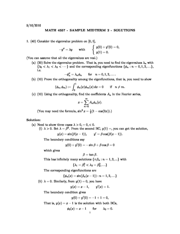
 1. (40) Consider the eigenvalue problem on [0, 1], −y 00 = λy with ( y(0) + y 0 (0) = 0, y(1) = 0. (You can assume that all the eigenvalues are real.) (a) (20) Solve the eigenvalue problem. That is, you need to find the eigenvalues λn with {λ0 < λ1 < λ2 < · · · } and the corresponding eigenfunctions {φn : n = 0, 1, 2, . . .}, i.e. −φ 00 n = λnφn for n = 0, 1, 2, . . . . (b) (10) Prove the orthogonality among the eigenfunctions, that is, you need to show (φn, φm) := Z 1 0 φn(x)φm(x) dx = 0 if n 6= m. (c) (10) Using the orthogonality, find the coefficients An in the Fourier series, x = X∞ n=0 Anφn(x). (You may need the formula, sin2 x = 1 2 (1 − cos(2x)).) Solution: (a) Need to show three cases λ > 0, = 0, < 0. (i) λ > 0. Set λ = β 2 . From the second BC, y(1) =, you can get the solution, y(x) = sin(β(x − 1)), y0 = β cos(β(x − 1)). The boundary conditions say y(0) + y 0 (0) = − sin β + β cos β = 0 which gives β = tan β. This has infinitely many solutions {±βn : n = 1, 2, ...} with {λ1 = β 2 1 < λ2 = β 2 2 , . . .} The corresponding eigenfunctions are {φn(x) = sin(βn(x − 1)) : n = 1, 2, . . .} (ii) λ = 0. Similarly, from y(1) = 0, you have y(x) = x − 1, y0 (x) = 1. The boundary condition gives y(0) + y 0 (0) = −1 + 1 = 0, That is, y(x) = x − 1 is the solution with both BCs, φ0(x) = x − 1 for λ0 = 0